You can run this notebook in a live session via Binder or view it on Github.

Contextual Median Filter

import matplotlib.pyplot as plt
import numpy as np
import xarray as xr
from fronts_toolbox._fields import (
    add_spikes,
    blobby_gradient,
    ideal_jet,
    sample,
    swap_noise,
)
from fronts_toolbox.filters import cmf_xarray

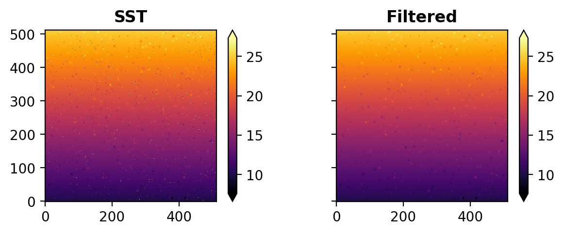
Blobby gradient

A gradient with blobs to preserve and spike noise.

sst_raw = blobby_gradient()
vmin = np.min(sst_raw)
vmax = np.max(sst_raw)
sst = xr.DataArray(
    add_spikes(sst_raw), name="sst", dims=("lat", "lon")
)
filtered = cmf_xarray(sst)

fig, axes = plt.subplots(
    1,
    2,
    figsize=(6, 2.3),
    layout="constrained",
    sharex=True,
    sharey=True,
    dpi=200,
)

im_kw = dict(
    cmap="inferno",
    add_labels=False,
    center=False,
    vmin=vmin,
    vmax=vmax,
)
sst.plot.imshow(ax=axes[0], **im_kw)
filtered.plot.imshow(ax=axes[1], **im_kw)

axes[0].set_title("SST", weight="bold")
axes[1].set_title("Filtered", weight="bold")

for ax in axes:
    ax.set_aspect("equal")

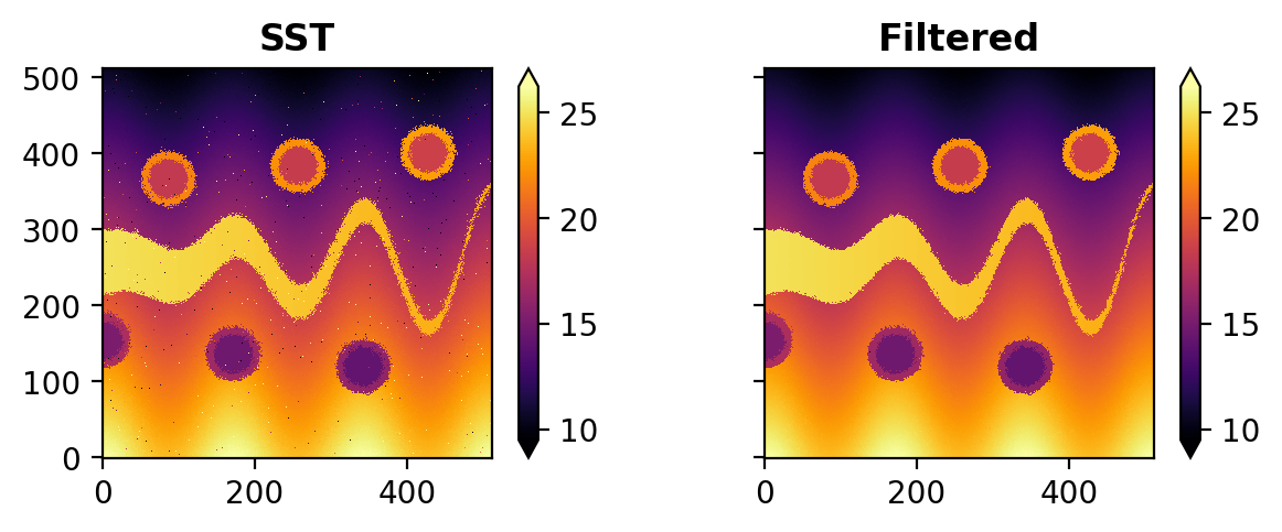
Ideal Jet

A idealized meandering jets with rings, as a 2D numpy array (embeded in Xarray) with swap noise and spikes.

sst_raw = ideal_jet()
vmin = np.min(sst_raw)
vmax = np.max(sst_raw)
sst = xr.DataArray(
    add_spikes(swap_noise(sst_raw)), name="sst", dims=("lat", "lon")
)
filtered = cmf_xarray(sst)

fig, axes = plt.subplots(
    1,
    2,
    figsize=(6, 2.3),
    layout="constrained",
    sharex=True,
    sharey=True,
    dpi=200,
)

im_kw = dict(
    cmap="inferno",
    add_labels=False,
    center=False,
    vmin=vmin,
    vmax=vmax,
)
sst.plot.imshow(ax=axes[0], **im_kw)
filtered.plot.imshow(ax=axes[1], **im_kw)

axes[0].set_title("SST", weight="bold")
axes[1].set_title("Filtered", weight="bold")

for ax in axes:
    ax.set_aspect("equal")

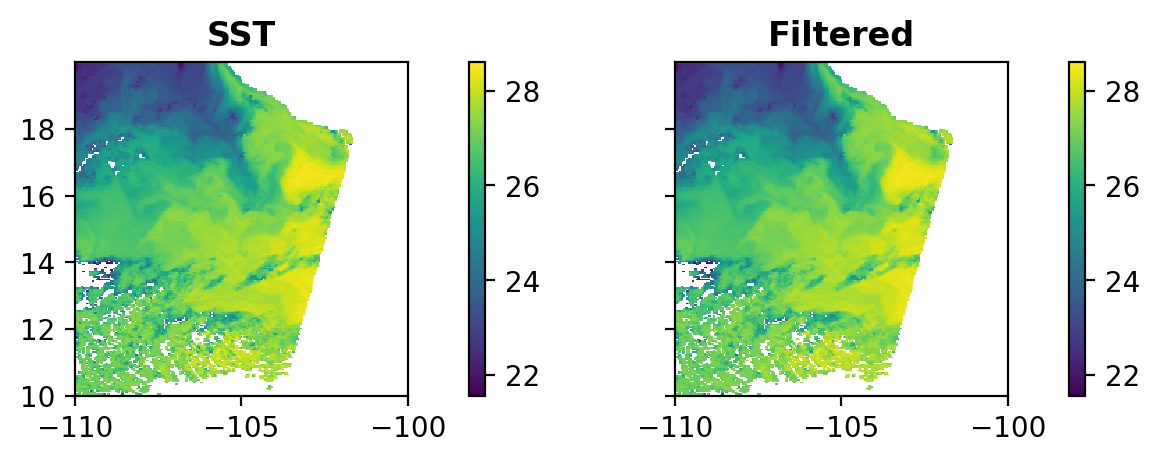
MODIS Data

SST off the Californian coast, as a Dask array embeded in Xarray.

sst = (
    sample("MODIS")
    .sst4.isel(time=0)
    .sel(lat=slice(20, 10), lon=slice(-110, -100))
    .chunk(lat=256, lon=256)
)
filtered = cmf_xarray(sst)

vmin = float(sst.min())
vmax = float(sst.max())

fig, axes = plt.subplots(
    1,
    2,
    figsize=(6, 2.2),
    layout="constrained",
    sharex=True,
    sharey=True,
    dpi=200,
)

im_kw = dict(
    add_labels=False,
    center=False,
    cbar_kwargs=dict(location="right", pad=0.05),
    vmin=vmin,
    vmax=vmax,
)
sst.plot.imshow(ax=axes[0], **im_kw)
filtered.plot.imshow(ax=axes[1], **im_kw)
axes[0].set_title("SST", weight="bold")
axes[1].set_title("Filtered", weight="bold")

for ax in axes:
    ax.set_aspect("equal")

/home/docs/checkouts/readthedocs.org/user_builds/fronts-toolbox/envs/stable/lib/python3.11/site-packages/fronts_toolbox/_fields.py:236: FutureWarning: In a future version of xarray the default value for data_vars will change from data_vars='all' to data_vars=None. This is likely to lead to different results when multiple datasets have matching variables with overlapping values. To opt in to new defaults and get rid of these warnings now use `set_options(use_new_combine_kwarg_defaults=True) or set data_vars explicitly.
  return xr.open_mfdataset(files, **kwargs)